Frigate Helipad – Structured O-H mesh

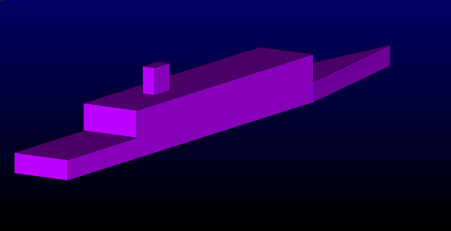
The May mesh showcases a fully structured O-H mesh of a frigate, called the Simple Frigate Shape (SFS2). SFS2 was meshed using an unstructured mesh in April. This month we are using the same SFS2 geometry, but instead of an unstructured mesh, we are meshing it fully structured with two alternative topologies:

1) a “H” mesh which resolves the boundary layer but does not wrap around the SFS2 surface (extends into farfield), and

2) an “O-H” body-wrapped mesh which also resolves the SFS2 boundary layer, but does wrap around the SFS2 surface.

Geometry

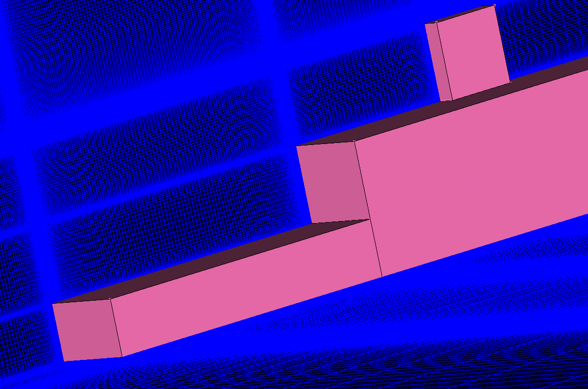
Figure 2 shows an overall view of the geometry. The farfield extents are sufficiently large to resolve the wake of the SFS2.

Like the unstructured mesh in April’s blog, the first cell height is 1.5cm, corresponding to a y+ of 100.

What are H and O-H Meshes?

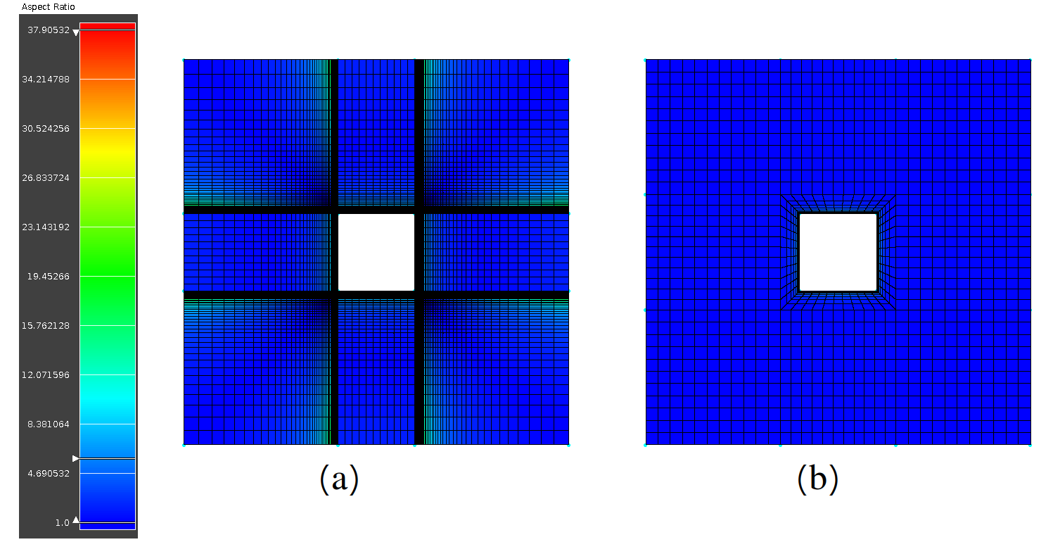
Lets go back one step – “H” and “O-H” meshes have been covered for cylindrical geometries (pipes etc) in previous Pointwise news and recently in a Tutorial Tuesday video. A square geometry (Figure 3(a)) can be meshed with a “H” topology, but this produces a high aspect ratio (maximum of 38 in the farfield), and has a relatively high number of elements (9680 hexa’s).

On the other hand a “O-H” wrapped mesh (Figure 3 (b)) produces a mesh with an aspect ratio maximum of 26, but this only occurs in the boundary layer, with the farfield close to aspect ratio 1. Furthermore only 1408 hexa elements are required.

Clearly the “O-H” mesh is better, but does require additional connectors offset from the body being wrapped to control the inflation. This has the benefit of allowing control of the viscous boundary layer with inflation.

H Structured Mesh for SFS2

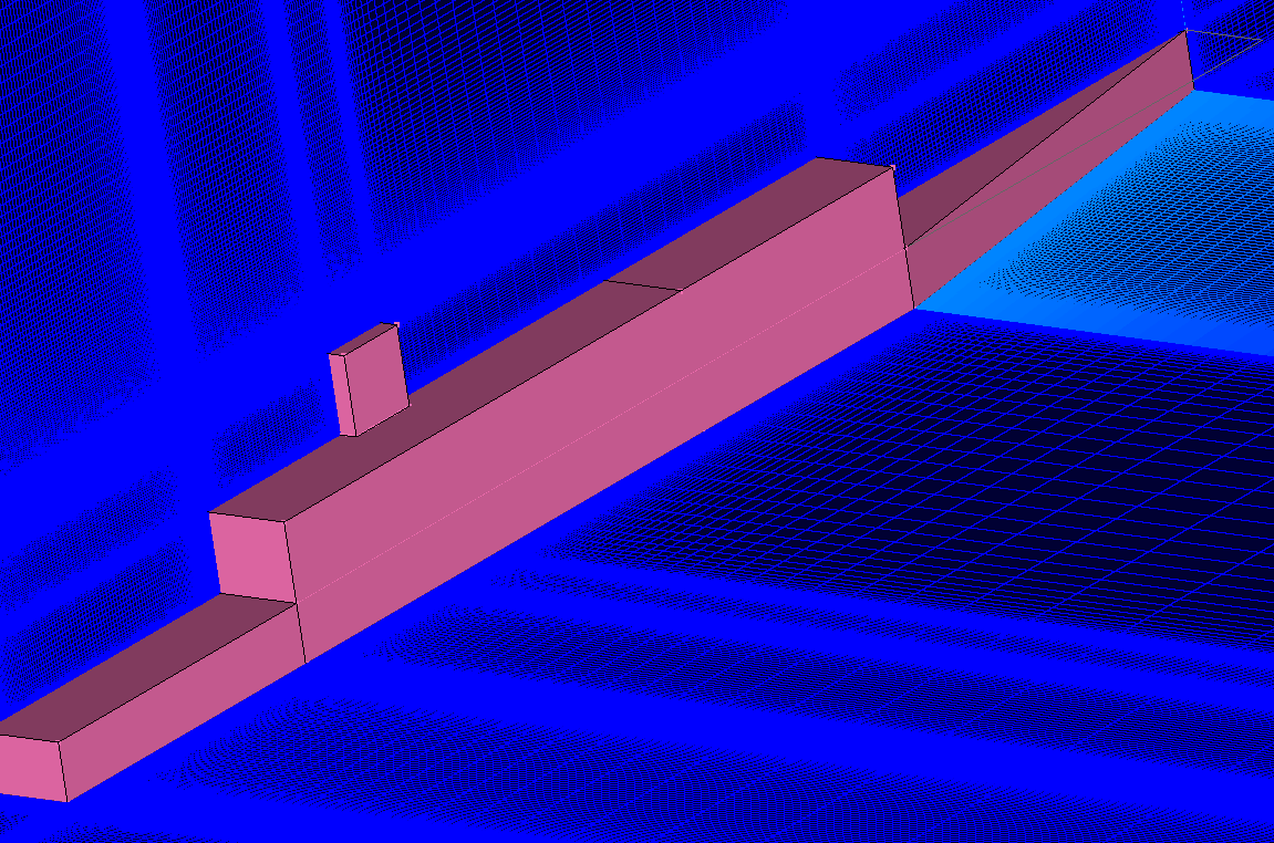
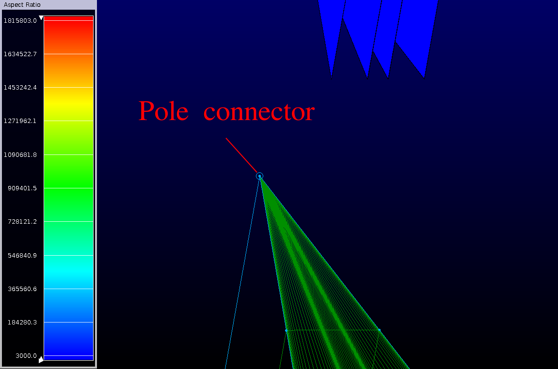
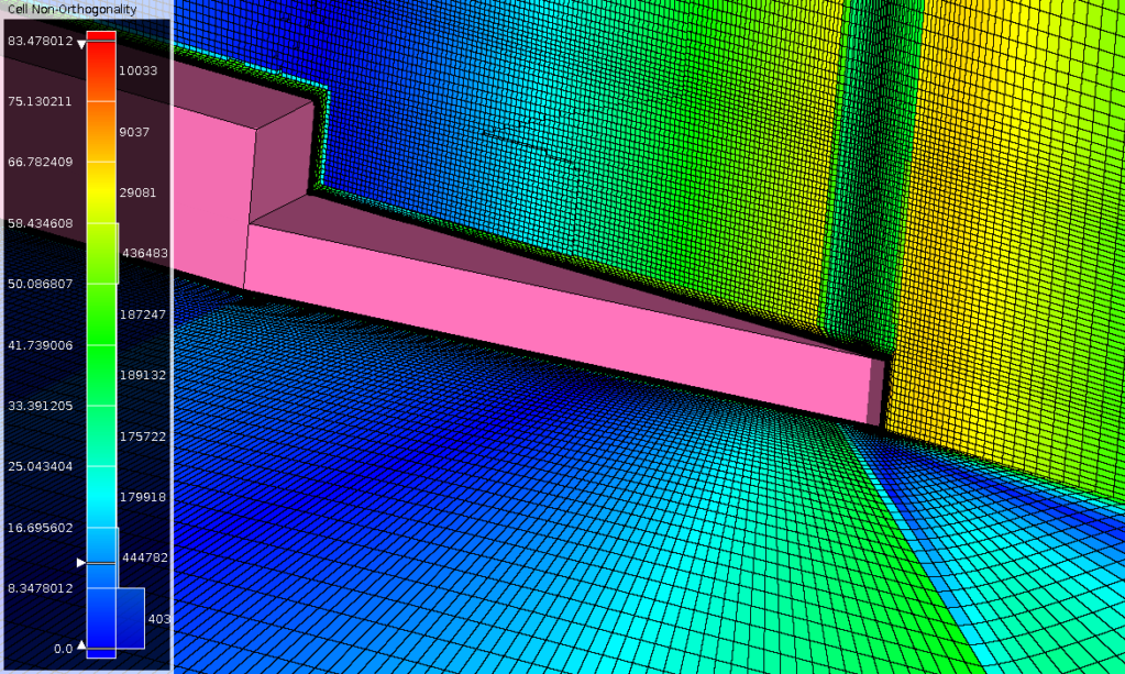
Since the boundary layer is refined, this refinement extends into the far-field for a “H” mesh. This is shown in Figures 4-5, resulting in very high aspect ratio cells. Around the nose of the SFS2 (Figure 6) pole connectors are used to deal with the triangular shape. Poles on triangular geometries were discussed in a recent Tutorial Tuesday video. Having poles can be problematic for some solvers since the elements created end up being as wedges. In this “H” mesh case, these elements extend into the farfield and cause the aspect ratio to be far too high (1,800,000) for most CFD solvers, due to these cells being in the free stream and not flow aligned.

An “O-H” mesh is discussed next, as it wraps around the user defined surfaces providing a boundary layer resolution without extending into the farfield.

O-H Structured Mesh for SFS2

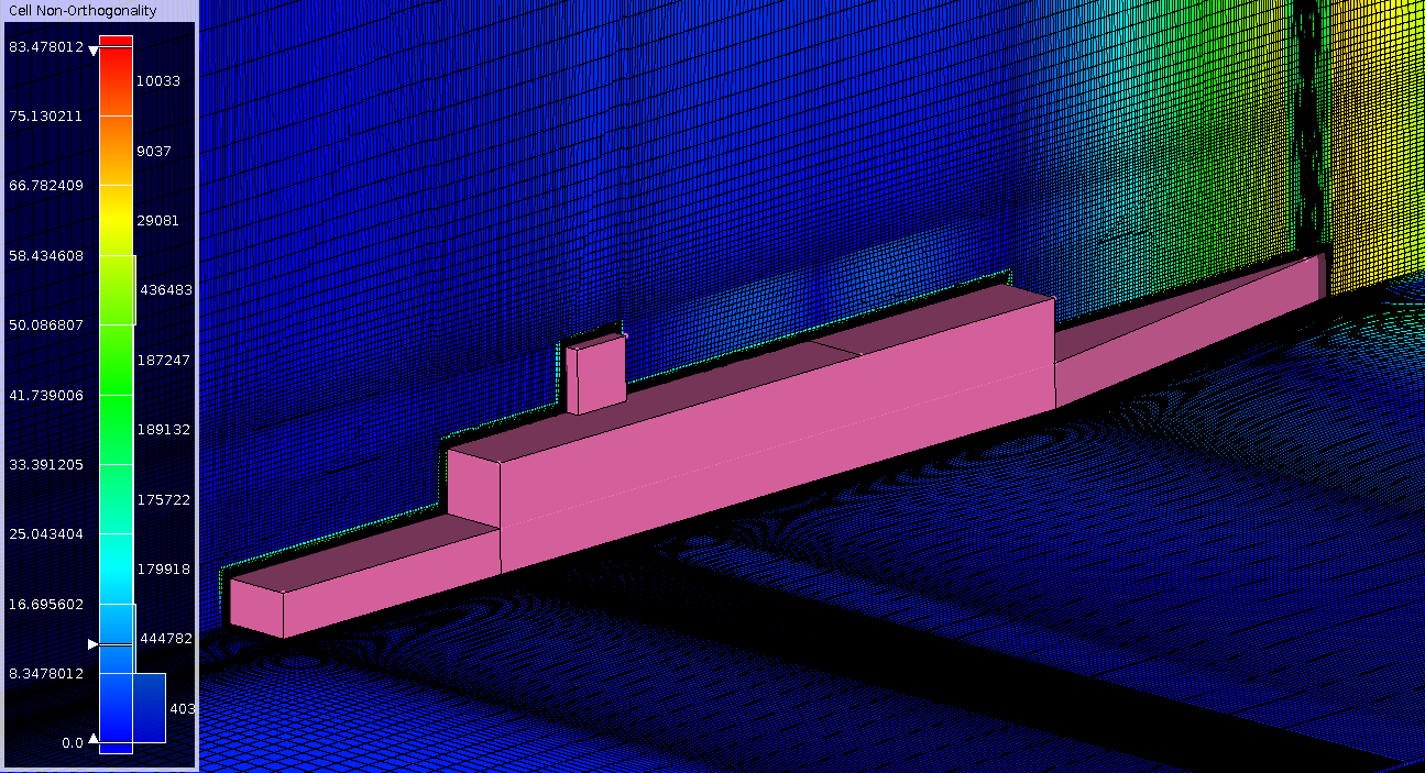
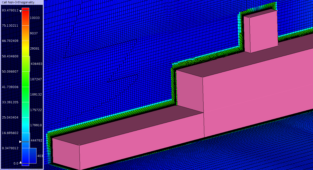
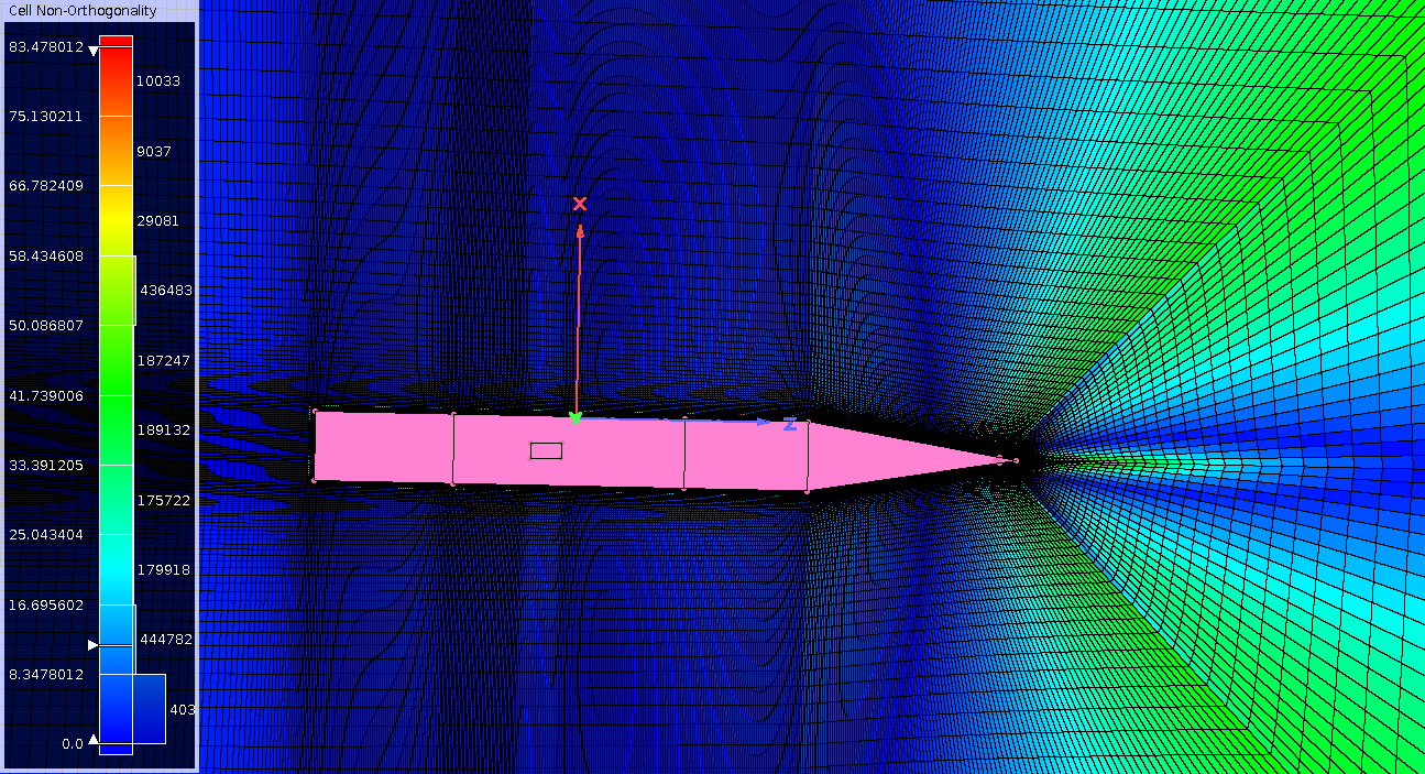
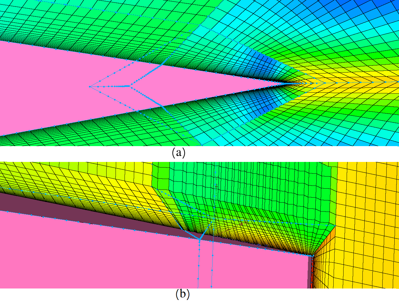
In Figures 7-11 the structured “O-H” mesh for the SFS2 is shown. The “O-H” topology wraps around the surface of the SFS2 using connectors offset at 45 degrees. A diamond topology is used to keep the cells as orthogonal as possible near the triangular nose.

“Breakpoints” were added to farfield connectors to control the splay from the SFS2 without requiring connectors to set the cell spacing distribution – this keeps the farfield mesh highly orthogonal. As a comparison to the “H” mesh and the unstructured mesh from the April blog, the mesh statistics are:

• The structured “O-H” mesh statistics: 8M elements with 100% hexa elements, max cell non-orthogonality of 82 degrees, aspect ratio of 102.
• The structured “H” mesh statistics: 49M elements with 100% hexa elements, max cell non-orthogonality of 72 degrees, aspect ratio of 1,800,000.
• The unstructured mesh statistics (April blog): 7.8M elements with 4.1M hexa, max cell non orthogonality of 87 degrees, aspect ratio of 240.

Although the “O-H” structured and unstructured meshes have a similar mesh size and quality metrics, the structured mesh is 100% hexa and generally more orthogonal (especially in the farfield), which is better for CFD solver accuracy. The “H” mesh has many more elements than the “O-H” and unstructured meshes, for the same first cell height and helideck cell edge length. This is due to the first cell height of 1.5cm extending into the farfield, which is the main detraction from “H” meshes.

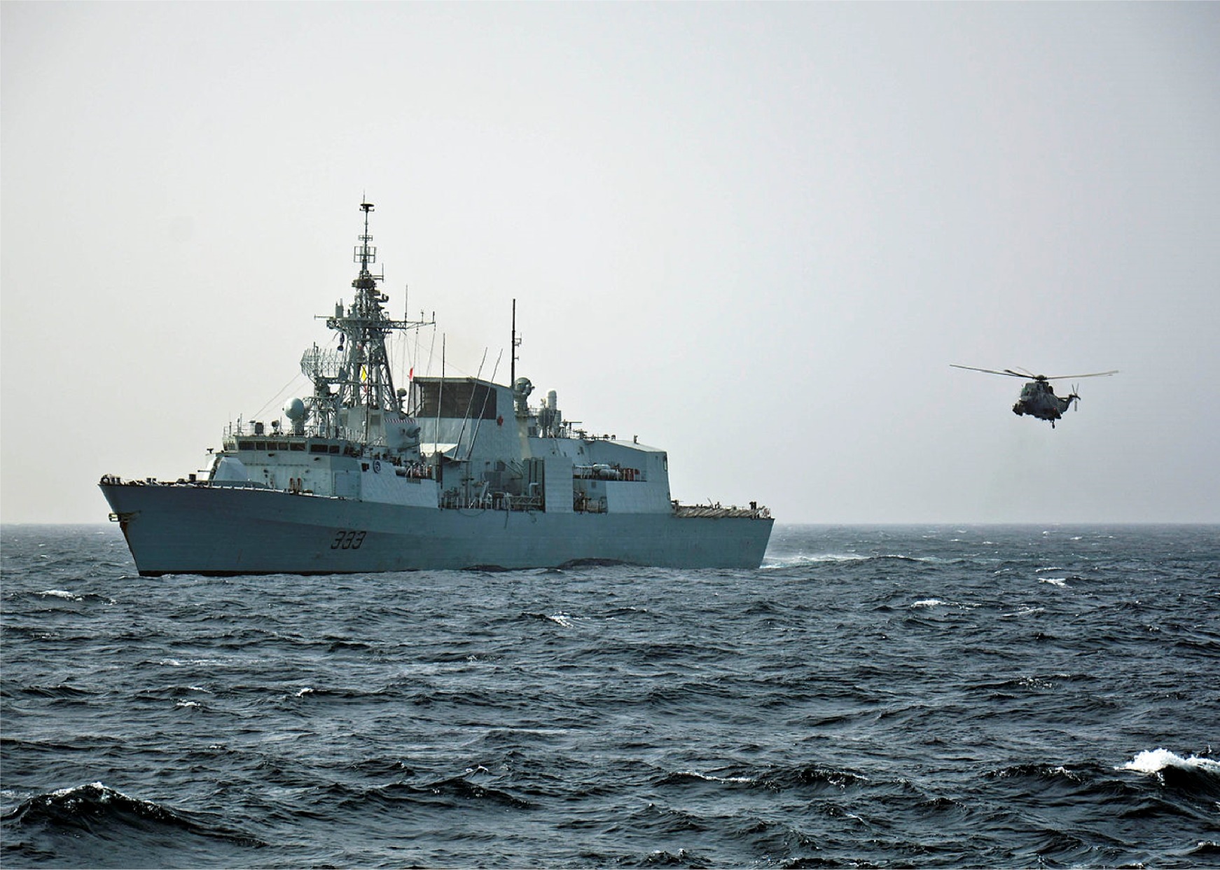
Where the unstructured mesh is favoured though is for more complex geometries, which cannot have a structured topology applied efficiently or at all. A real frigate has additional features (over the SFS2), such as deck equipment, hand railings and general bluff bodies upstream of the helipad. These would need to be modelled to correctly predict turbulence at the helideck. These details can be critical, and in some countries the modelling of fluctuations in velocity have guidelines. In the UK, Civil Aviation guidelines state that “As a general rule, a limit on the standard deviation of the vertical airflow velocity of 1.75 m/s should not be exceeded” (Ref [1]).

In case you missed it…

Check out last month’s mesh if you missed it!

Thanks for reading, the next edition will be June 2019. Until then, happy meshing!

For a free trial of Pointwise, go here.

References:

[1] Standards for offshore helicopter landing areas
CAP 437 https://www.aspa.com.my/download/UK-CAP-437.pdf, Civil Aviation Authority, 2016